Challenge 03
Due: 2025-04-24 at the start of class
Download Starter Files Submit on GradescopeWe will review revisions of challenges on a rolling basis, and if you submit early you may have a chance to go through multiple revision cycles. As students often submit work that is not finalized to gradescope, we ask that you fill out this form to indicate that your submission is ready to be regraded.
Objectives
- Demonstrate your ability to design and write a program on your own
- Demonstrate your ability to work with two dimensional data
- Demonstrate your ability to implement a mathematical algorithm
Challenges
Challenges are your moment to demonstrate your ability to apply the concepts from the class independently. We may provide a framework that allows us to test your code and a description of the problem to be solved. The design of that solution is left up to you. We will not tell you how many functions to write, their names or what their parameters should be, nor will we dictate any implementation details beyond the requirements placed on what data you wll be given and what form we expect any data to be output. The only requirement is that your submission be entirely your own work.
Requirements
Challenges will only be marked Satisfactory, Incomplete or Unassessable.
To be marked Satisfactory,
- your code must meet the functional requirements (as embodied by the tests of Gradescope)
- your code must pass the style tests
- any function you write must have well formed docstrings that describe the purpose of the function, the name and type of each parameter and the return value
- your design should demonstrate good choices with respect to choices of abstraction and implementation (i.e., what to create as a function, how to handle repetition, how to break up conditions, etc…)
There are many ways to demonstrate good choices. At the largest scale, we will looking at how you use abstraction. Your functions should just do one thing, and that thing should make sense as a part of the problem you are solving. If you can’t describe what your function does in a simple sentence, it is probably too complex. On a small scale, good choices illustrate your grasp of how your tools work. For example, we might look at unnecessary type conversions (like converting a string literal to a string, e.g., str("already a string")).
Submissions that are marked Incomplete will be eligible to be revised after feedback is returned. New work, or work that is Unassessable when the first submission period closes will not be accepted for revisions.
The Problem
For this challenge your task is to create an image with a collection of colored lines drawn on it. As with the other challenges, to provide you with the maximum amount of flexibility and still allow us to auto-grade your work, you will read in directions from a configuration file.
(please read all of this page before starting to implement this – we have a very specific way to handle the file operations).
Drawing lines
Drawing lines that either have no change in x or no change in y is pretty straightforward. You just need to figure out which dimension is changing and then iterate over the points in the other dimension, coloring them in.
Things get more complicated (interesting) when the lines connect to arbitrary points on the image. The problem is that lines are (mathematically at least) infinitely thin, but we need to draw by filling in pixels. One way to imagine this problem is to take a sheet of graph paper and then draw a thin line on top of it. You then want to fill in the squares on the graph paper that most closely approximate the line you drew. To make the line look nice, it should be connected (every pixel touches its two neighbors - even if it is just corner to corner) but we don’t want the line to have clumps where the line gets thicker.
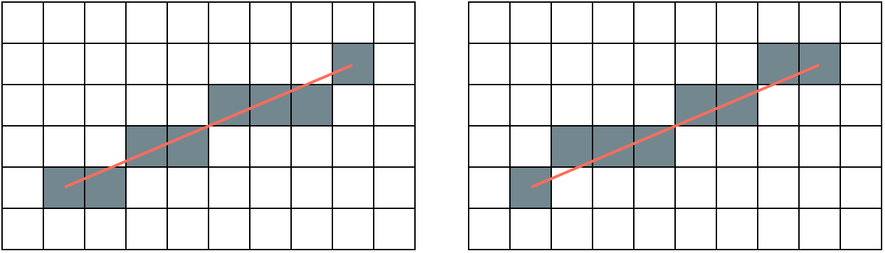
Both of these solutions approximate the line (in red), though one is perhaps a little better than the other.
This is an old problem and there are a couple of classic algorithms. We aren’t going to use the fastest and cleverest one – we are going to prioritize conceptual simplicity over cleverness.
The mid-point algorithm
Background
We are going to use something called the mid-point algorithm.
For the description of the algorithm, we will consider two points (\((x_0, y_0)\) and \((x_1, y_1)\)). Assume that \(x_0 < x_1\).
Guaranteeing that \(x_0 < x_1\) is pretty straightforward. If condition isn’t met, just swap the two values. We don’t really care which end of the line is the “start”.
We will make a further stipulation about our line. The slope of the line \(m\), is given by \[ m = \frac{y_1 - y_0}{x_1 - x_0} \]
For the rest of the discussion of the algorithm, we will assume that \(m \in(0, 1]\). To say that with less math, both \(x\) and \(y\) are increasing and \(x\) is increasing faster than \(y\).
Another piece that we need is the implicit function for a line.
\[ f(x, y) = (x_1 - x_0)y - (y_1 - y_0)x + x_0y_1 - x_1y_0 = 0 \]
What in the world does all of that mean!? I will spare you the derivation. The point here is that we have a line defined by two end points (\((x_0, y_0)\) and \((x_1, y_1)\)). I can test a new point \((x, y)\) by plugging it into this equation. If the result is zero, then the point \((x, y)\) is on the line. If the result is not zero, then the sign of the result can tell us which side of the line we are on. A positive result means that the point is over the line. A negative result says the point is under the line.
So, to recap: - we have two points \((x_0, y_0)\) and \((x_1, y_1)\) - \(x_0 < x_1\) - the change in \(x\) is greater than or equal to the change in \(y\) - we have a function that will tell us if a point is on the line, above it or below it
The algorithm
The core of the algorithm is an iteration over the values of x from x0 to x1. Since x is changing more than y, we can just march one pixel at a time in the x direction. If we get too far off the line we are trying to draw, we increment y.
In pseudocode:
y = y0
for x in x0 to x1
    fill in pixel x,y
    if drawing the next pixel would take us too far away from the line
        y += 1
Obviously the stickler is that condition. This is where the “midpoint” part of the algorithm comes in.
Consider the following
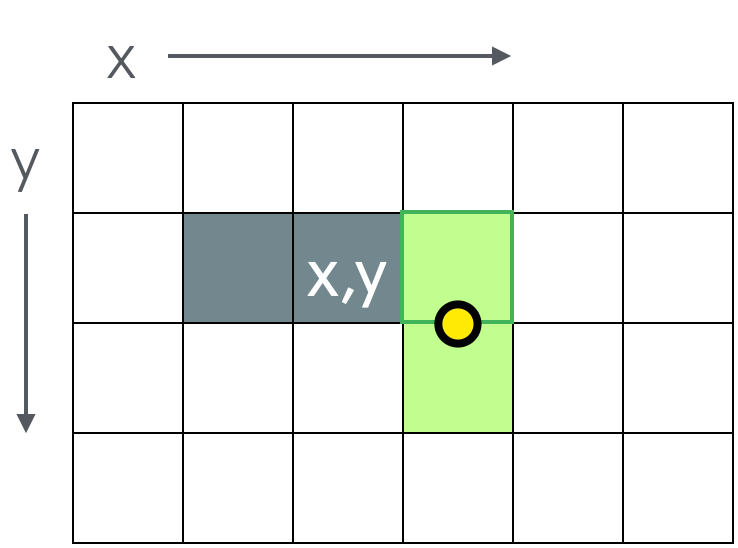
You have just drawn point \((x, y)\). You are trying to decide which of the green squares to move to next (remember that \(y\) increases down). The two candidate squares are \((x + 1, y)\) (top) and \((x + 1, y + 1)\) (bottom).
To answer the questions we are going to look at the midpoint (the yellow dot). This is the point \((x + 1, y + 0.5)\). This is where our implicit equation for the line comes in. We pass it the midpoint. There are now three options, the result is 0 (the line runs right through the midpoint and it doesn’t matter which square we pick), the result is positive or the result is negative.
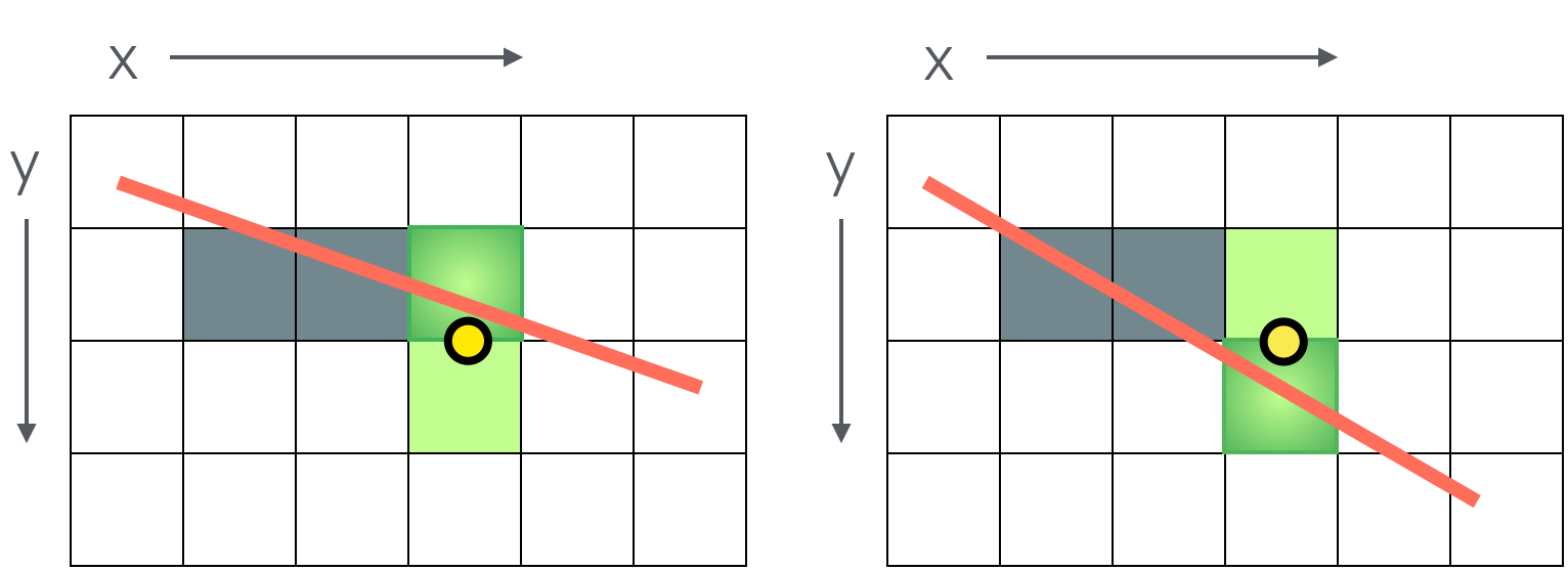
If the result is positive, then the midpoint is over the line (closer to the bottom as in the left image). If the result is negative, then the midpoint is under the line (closer to the top as in the right image). So, we want to increment y when the result is negative and leave it alone when the result is positive.
That’s it. That’s the algorithm. There are some fancier versions that are faster because they do less math and do everything with integers, but we aren’t doing anything serious enough to worry about speed and this version is easier to understand.
The octants
Okay, that wasn’t exactly a lie, but it wasn’t the whole picture (so to speak).
Recall the set of assumptions we started with:
- \(x_0 < x_1\)
- the change in \(x\) is greater than or equal to the change in \(y\)
This covers only a fraction of the possible lines we might want to draw (slightly less than 1/8th of them).
Starting from \(x_0\), if we were to imagine all possible lines of a certain length, the endpoints of those lines would form a circle around \(x_0\). The region we have covered is the region in blue.
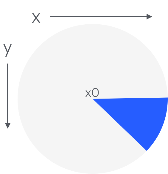
To cover the rest of the regions, we need to consider what \(x\) and \(y\) are doing in each one.
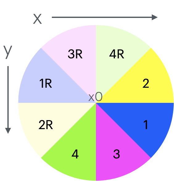
| Region | \(x\) behavior | \(y\) behavior | changing faster |
|---|---|---|---|
| 1 | increasing | increasing | \(x\) |
| 1R | decreasing | decreasing | \(x\) |
| 2 | increasing | decreasing | \(x\) |
| 2R | decreasing | increasing | \(x\) |
| 3 | increasing | increasing | \(y\) |
| 3R | decreasing | decreasing | \(y\) |
| 4 | decreasing | increasing | \(y\) |
| 4R | increasing | decreasing | \(y\) |
Reflections
The first thing to notice is the “R” regions. These are the regions where the faster changing variable goes in the other direction. All of these can be addressed by flipping the end points when appropriate.
Region 2
Region 2 requires the least amount of change from the algorithm. Instead of increasing, \(y\) should decrease when we do the correction step. Also consider that the correction step will work in the opposite direction.
Regions 3 and 4
Regions 3 and 4 are variations of regions 1 and 2. The difference is that now \(y\) is the faster changing variable, so we need to flip the algorithm to iterate by \(y\) instead of \(x\) and change the midpoint test and course correction appropriately as well.
Special cases - changing at the same rate
In the cases where \(x\) and \(y\) are changing at exactly the same rate, use the increment by \(x\) part of your code. Conceptually it should produce identical results, but you will need to pick one.
Special cases - horizontal and vertical lines
Horizontal and vertical lines are special because there is no change in one of the two variables. It is worth treating these as special cases for a couple of reasons. First, it is just more efficient to draw these simple lines without doing all of the line testing. Second, if you are calculating the slope, you will have an issue if there is no change in \(y\).
Details
We want to give you the maximum amount of flexibility with this challenge while still retaining the ability to provide you with on demand feedback with the autograder, so we have had to give you a little bit of a framework to support these two competing demands.
main()
In the starter code (challenge03.py), you will see the following code:
import task_handler


def main():
    """
    This is the "main" function that drives your program. This is the function we will call when we want to run your code.
    """
    config = task_handler.get_configuration()
Once again, you will be writing a program that carries out multiple operations. Programs typically have a function called main that serves as the entry point – where the first instruction to run is found. This is the function we will call to run your code.
A good solution to this challenge is unlikely to put all of its code in main() (very unlikely…). You can, of course, test any function you write independently of main, but bear in mind that we won’t know what your functions are, so we will only run main.
Because of the nature of the autograder, please do not leave a call to main() in your file.
Configuration
The configuration given to you by task_handler.get_configuration() will be a dictionary with the same structure as the contents of configuration.json. You should familiarize yourself with that file (and later edit it for testing).
The configuration dictionary has two keys: dimensions and lines.
The dimensions will be another dictionary with keys width and height. Both of these should have integer values. These dimensions should be used as the dimensions of the image you create.
lines is a list of dictionaries – one per line you need to draw. Each line has three keys: start, end, and color.
Both start and end store dictionaries with keys x and y. The associated values are integers.
The color key maps to a string containing a hexstring formatted color (e.g. `“#003479” – aka “Middlebury Blue”).
task_handler.get_configuration() takes and optional file name. It would be a good idea to have a couple of different configurations that allow you to test different parts of your solution.
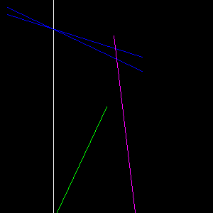
Here is a sample configuration file. I have colored the lines to align to the quadrant colors above. Note that this is not a comprehensive set of tests. You absolutely should make some of your own.
{
  "dimensions": {"width": 300, "height": 300},
  "lines": [
    {"start": {"x": 75, "y": 0}, "end": {"x": 75, "y": 299}, "color": "#FFFFFF"},
    {"start": {"x": 10, "y": 10}, "end": {"x": 200, "y": 100}, "color": "#0000FF"},
    {"start": {"x": 10, "y": 20}, "end": {"x": 200, "y": 80}, "color": "#0000FF"},
    {"start": {"x": 150, "y": 150}, "end": {"x": 80, "y": 299}, "color": "#00FF00"},
    {"start": {"x": 160, "y": 50}, "end": {"x": 190, "y": 299}, "color": "#FF00FF"}
  ]
}
Output
When you have drawn all of the lines, call task_handler.submit() and pass it your image. This will call show() on your image and display it to you. While not visible in the code, the autograder will detect the submission and run its checks on the image you submit.
Submission
As usual, you are encouraged to submit early and often to test your work against the autograder. The only file that you need to submit is challenge03.py (and any other files you may have written as part of your solution). You do not need to submit input or output files, nor do we need task_handler.py.