nonlinear-fitting

Nonlinear Fitting and Convexity

Consider ‍‍‍‍‍‍‍‍‍‍‍‍‍‍‍‍‍‍‍‍the ‍‍‍‍‍‍‍‍‍‍‍‍‍‍‍‍‍‍‍‍nonlinear ‍‍‍‍‍‍‍‍‍‍‍‍‍‍‍‍‍‍‍‍regression ‍‍‍‍‍‍‍‍‍‍‍‍‍‍‍‍‍‍‍‍model ‍‍‍‍‍‍‍‍‍‍‍‍‍‍‍‍‍‍‍‍in ‍‍‍‍‍‍‍‍‍‍‍‍‍‍‍‍‍‍‍‍1D ‍‍‍‍‍‍‍‍‍‍‍‍‍‍‍‍‍‍‍‍in ‍‍‍‍‍‍‍‍‍‍‍‍‍‍‍‍‍‍‍‍which ‍‍‍‍‍‍‍‍‍‍‍‍‍‍‍‍‍‍‍‍the ‍‍‍‍‍‍‍‍‍‍‍‍‍‍‍‍‍‍‍‍score ‍‍‍‍‍‍‍‍‍‍‍‍‍‍‍‍‍‍‍‍for ‍‍‍‍‍‍‍‍‍‍‍‍‍‍‍‍‍‍‍‍a ‍‍‍‍‍‍‍‍‍‍‍‍‍‍‍‍‍‍‍‍data ‍‍‍‍‍‍‍‍‍‍‍‍‍‍‍‍‍‍‍‍point ‍‍‍‍‍‍‍‍‍‍‍‍‍‍‍‍‍‍‍‍\(i\) ‍‍‍‍‍‍‍‍‍‍‍‍‍‍‍‍‍‍‍‍is ‍‍‍‍‍‍‍‍‍‍‍‍‍‍‍‍‍‍‍‍computed ‍‍‍‍‍‍‍‍‍‍‍‍‍‍‍‍‍‍‍‍according ‍‍‍‍‍‍‍‍‍‍‍‍‍‍‍‍‍‍‍‍to ‍‍‍‍‍‍‍‍‍‍‍‍‍‍‍‍‍‍‍‍the ‍‍‍‍‍‍‍‍‍‍‍‍‍‍‍‍‍‍‍‍formula

\[ \begin{aligned} s_i = f_{\mathbf{w},\gamma}(x_i) = w_1x_i^{\gamma} + w_0\;. \end{aligned} \]

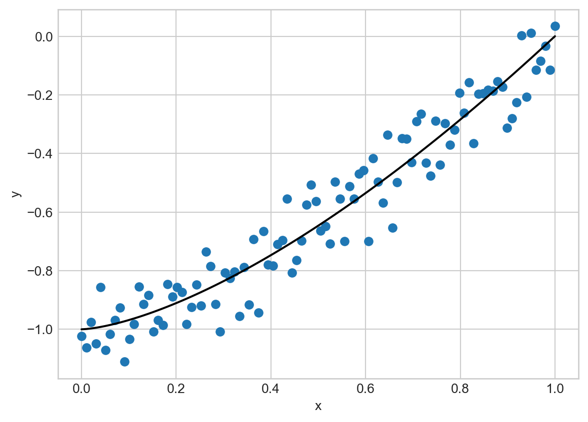
If ‍‍‍‍‍‍‍‍‍‍‍‍‍‍‍‍‍‍‍‍all ‍‍‍‍‍‍‍‍‍‍‍‍‍‍‍‍‍‍‍‍we ‍‍‍‍‍‍‍‍‍‍‍‍‍‍‍‍‍‍‍‍wanted ‍‍‍‍‍‍‍‍‍‍‍‍‍‍‍‍‍‍‍‍to ‍‍‍‍‍‍‍‍‍‍‍‍‍‍‍‍‍‍‍‍learn ‍‍‍‍‍‍‍‍‍‍‍‍‍‍‍‍‍‍‍‍was ‍‍‍‍‍‍‍‍‍‍‍‍‍‍‍‍‍‍‍‍\(\mathbf{w}\) ‍‍‍‍‍‍‍‍‍‍‍‍‍‍‍‍‍‍‍‍in ‍‍‍‍‍‍‍‍‍‍‍‍‍‍‍‍‍‍‍‍this ‍‍‍‍‍‍‍‍‍‍‍‍‍‍‍‍‍‍‍‍model, ‍‍‍‍‍‍‍‍‍‍‍‍‍‍‍‍‍‍‍‍we ‍‍‍‍‍‍‍‍‍‍‍‍‍‍‍‍‍‍‍‍could ‍‍‍‍‍‍‍‍‍‍‍‍‍‍‍‍‍‍‍‍use ‍‍‍‍‍‍‍‍‍‍‍‍‍‍‍‍‍‍‍‍standard ‍‍‍‍‍‍‍‍‍‍‍‍‍‍‍‍‍‍‍‍tools ‍‍‍‍‍‍‍‍‍‍‍‍‍‍‍‍‍‍‍‍that ‍‍‍‍‍‍‍‍‍‍‍‍‍‍‍‍‍‍‍‍we’ve ‍‍‍‍‍‍‍‍‍‍‍‍‍‍‍‍‍‍‍‍seen ‍‍‍‍‍‍‍‍‍‍‍‍‍‍‍‍‍‍‍‍previously. ‍‍‍‍‍‍‍‍‍‍‍‍‍‍‍‍‍‍‍‍However, ‍‍‍‍‍‍‍‍‍‍‍‍‍‍‍‍‍‍‍‍suppose ‍‍‍‍‍‍‍‍‍‍‍‍‍‍‍‍‍‍‍‍that ‍‍‍‍‍‍‍‍‍‍‍‍‍‍‍‍‍‍‍‍we ‍‍‍‍‍‍‍‍‍‍‍‍‍‍‍‍‍‍‍‍would ‍‍‍‍‍‍‍‍‍‍‍‍‍‍‍‍‍‍‍‍also ‍‍‍‍‍‍‍‍‍‍‍‍‍‍‍‍‍‍‍‍like ‍‍‍‍‍‍‍‍‍‍‍‍‍‍‍‍‍‍‍‍to ‍‍‍‍‍‍‍‍‍‍‍‍‍‍‍‍‍‍‍‍learn ‍‍‍‍‍‍‍‍‍‍‍‍‍‍‍‍‍‍‍‍\(\gamma\). ‍‍‍‍‍‍‍‍‍‍‍‍‍‍‍‍‍‍‍‍Here’s ‍‍‍‍‍‍‍‍‍‍‍‍‍‍‍‍‍‍‍‍an ‍‍‍‍‍‍‍‍‍‍‍‍‍‍‍‍‍‍‍‍example ‍‍‍‍‍‍‍‍‍‍‍‍‍‍‍‍‍‍‍‍of ‍‍‍‍‍‍‍‍‍‍‍‍‍‍‍‍‍‍‍‍this ‍‍‍‍‍‍‍‍‍‍‍‍‍‍‍‍‍‍‍‍model ‍‍‍‍‍‍‍‍‍‍‍‍‍‍‍‍‍‍‍‍when ‍‍‍‍‍‍‍‍‍‍‍‍‍‍‍‍‍‍‍‍\(\mathbf{w} = (1, -1)\) ‍‍‍‍‍‍‍‍‍‍‍‍‍‍‍‍‍‍‍‍and ‍‍‍‍‍‍‍‍‍‍‍‍‍‍‍‍‍‍‍‍\(\gamma = 1.5\):

Code

import torch 
from matplotlib import pyplot as plt
plt.style.use('seaborn-v0_8-whitegrid')

def poly_model(X, w = torch.tensor([1, -1]), gamma = torch.tensor([1.5])):

    return w[0] * X**gamma[0] + w[1]

def create_data(n = 100, w = torch.tensor([1, -1]), gamma = torch.tensor([1.5])):
    """
    Create a dataset with n samples and gamma features. 
    """
    X = torch.linspace(0, 1, n).reshape(-1, 1)
    y = poly_model(X, w, gamma) + 0.1*torch.randn(n, 1)
    return X, y

X, y = create_data()
plt.scatter(X, y)
x = torch.linspace(0, 1, 100).reshape(-1, 1)
plt.plot(x, poly_model(x), color = "black", )
plt.gca().set(xlabel = "x", ylabel = "y")

To ‍‍‍‍‍‍‍‍‍‍‍‍‍‍‍‍‍‍‍‍determine ‍‍‍‍‍‍‍‍‍‍‍‍‍‍‍‍‍‍‍‍the ‍‍‍‍‍‍‍‍‍‍‍‍‍‍‍‍‍‍‍‍optimal ‍‍‍‍‍‍‍‍‍‍‍‍‍‍‍‍‍‍‍‍parameters ‍‍‍‍‍‍‍‍‍‍‍‍‍‍‍‍‍‍‍‍\(\mathbf{w}\) ‍‍‍‍‍‍‍‍‍‍‍‍‍‍‍‍‍‍‍‍and ‍‍‍‍‍‍‍‍‍‍‍‍‍‍‍‍‍‍‍‍\(\gamma\), ‍‍‍‍‍‍‍‍‍‍‍‍‍‍‍‍‍‍‍‍we’ll ‍‍‍‍‍‍‍‍‍‍‍‍‍‍‍‍‍‍‍‍choose ‍‍‍‍‍‍‍‍‍‍‍‍‍‍‍‍‍‍‍‍the ‍‍‍‍‍‍‍‍‍‍‍‍‍‍‍‍‍‍‍‍same ‍‍‍‍‍‍‍‍‍‍‍‍‍‍‍‍‍‍‍‍squared-error ‍‍‍‍‍‍‍‍‍‍‍‍‍‍‍‍‍‍‍‍loss ‍‍‍‍‍‍‍‍‍‍‍‍‍‍‍‍‍‍‍‍function ‍‍‍‍‍‍‍‍‍‍‍‍‍‍‍‍‍‍‍‍that ‍‍‍‍‍‍‍‍‍‍‍‍‍‍‍‍‍‍‍‍we ‍‍‍‍‍‍‍‍‍‍‍‍‍‍‍‍‍‍‍‍used ‍‍‍‍‍‍‍‍‍‍‍‍‍‍‍‍‍‍‍‍in ‍‍‍‍‍‍‍‍‍‍‍‍‍‍‍‍‍‍‍‍other ‍‍‍‍‍‍‍‍‍‍‍‍‍‍‍‍‍‍‍‍regression ‍‍‍‍‍‍‍‍‍‍‍‍‍‍‍‍‍‍‍‍problems:

\[ \begin{aligned} L(\mathbf{w}, \gamma) = \frac{1}{n}\sum_{i=1}^n (y_i - f_{\mathbf{w},\gamma}(x_i))^2\;. \end{aligned} \]

Part A

Please ‍‍‍‍‍‍‍‍‍‍‍‍‍‍‍‍‍‍‍‍determine ‍‍‍‍‍‍‍‍‍‍‍‍‍‍‍‍‍‍‍‍the ‍‍‍‍‍‍‍‍‍‍‍‍‍‍‍‍‍‍‍‍gradient ‍‍‍‍‍‍‍‍‍‍‍‍‍‍‍‍‍‍‍‍of ‍‍‍‍‍‍‍‍‍‍‍‍‍‍‍‍‍‍‍‍this ‍‍‍‍‍‍‍‍‍‍‍‍‍‍‍‍‍‍‍‍loss ‍‍‍‍‍‍‍‍‍‍‍‍‍‍‍‍‍‍‍‍function, ‍‍‍‍‍‍‍‍‍‍‍‍‍‍‍‍‍‍‍‍including ‍‍‍‍‍‍‍‍‍‍‍‍‍‍‍‍‍‍‍‍the ‍‍‍‍‍‍‍‍‍‍‍‍‍‍‍‍‍‍‍‍partial ‍‍‍‍‍‍‍‍‍‍‍‍‍‍‍‍‍‍‍‍derivative ‍‍‍‍‍‍‍‍‍‍‍‍‍‍‍‍‍‍‍‍with ‍‍‍‍‍‍‍‍‍‍‍‍‍‍‍‍‍‍‍‍respect ‍‍‍‍‍‍‍‍‍‍‍‍‍‍‍‍‍‍‍‍to ‍‍‍‍‍‍‍‍‍‍‍‍‍‍‍‍‍‍‍‍\(\gamma\). ‍‍‍‍‍‍‍‍‍‍‍‍‍‍‍‍‍‍‍‍You ‍‍‍‍‍‍‍‍‍‍‍‍‍‍‍‍‍‍‍‍may ‍‍‍‍‍‍‍‍‍‍‍‍‍‍‍‍‍‍‍‍find ‍‍‍‍‍‍‍‍‍‍‍‍‍‍‍‍‍‍‍‍the ‍‍‍‍‍‍‍‍‍‍‍‍‍‍‍‍‍‍‍‍other ‍‍‍‍‍‍‍‍‍‍‍‍‍‍‍‍‍‍‍‍partial ‍‍‍‍‍‍‍‍‍‍‍‍‍‍‍‍‍‍‍‍derivatives ‍‍‍‍‍‍‍‍‍‍‍‍‍‍‍‍‍‍‍‍to ‍‍‍‍‍‍‍‍‍‍‍‍‍‍‍‍‍‍‍‍be ‍‍‍‍‍‍‍‍‍‍‍‍‍‍‍‍‍‍‍‍similar ‍‍‍‍‍‍‍‍‍‍‍‍‍‍‍‍‍‍‍‍to ‍‍‍‍‍‍‍‍‍‍‍‍‍‍‍‍‍‍‍‍a ‍‍‍‍‍‍‍‍‍‍‍‍‍‍‍‍‍‍‍‍problem ‍‍‍‍‍‍‍‍‍‍‍‍‍‍‍‍‍‍‍‍that ‍‍‍‍‍‍‍‍‍‍‍‍‍‍‍‍‍‍‍‍we’ve ‍‍‍‍‍‍‍‍‍‍‍‍‍‍‍‍‍‍‍‍done ‍‍‍‍‍‍‍‍‍‍‍‍‍‍‍‍‍‍‍‍before.

Part B

Take ‍‍‍‍‍‍‍‍‍‍‍‍‍‍‍‍‍‍‍‍the ‍‍‍‍‍‍‍‍‍‍‍‍‍‍‍‍‍‍‍‍second ‍‍‍‍‍‍‍‍‍‍‍‍‍‍‍‍‍‍‍‍derivative ‍‍‍‍‍‍‍‍‍‍‍‍‍‍‍‍‍‍‍‍of ‍‍‍‍‍‍‍‍‍‍‍‍‍‍‍‍‍‍‍‍the ‍‍‍‍‍‍‍‍‍‍‍‍‍‍‍‍‍‍‍‍loss ‍‍‍‍‍‍‍‍‍‍‍‍‍‍‍‍‍‍‍‍with ‍‍‍‍‍‍‍‍‍‍‍‍‍‍‍‍‍‍‍‍respect ‍‍‍‍‍‍‍‍‍‍‍‍‍‍‍‍‍‍‍‍to ‍‍‍‍‍‍‍‍‍‍‍‍‍‍‍‍‍‍‍‍\(\gamma\), ‍‍‍‍‍‍‍‍‍‍‍‍‍‍‍‍‍‍‍‍for ‍‍‍‍‍‍‍‍‍‍‍‍‍‍‍‍‍‍‍‍fixed ‍‍‍‍‍‍‍‍‍‍‍‍‍‍‍‍‍‍‍‍\(\mathbf{w}\). ‍‍‍‍‍‍‍‍‍‍‍‍‍‍‍‍‍‍‍‍Is ‍‍‍‍‍‍‍‍‍‍‍‍‍‍‍‍‍‍‍‍the ‍‍‍‍‍‍‍‍‍‍‍‍‍‍‍‍‍‍‍‍loss ‍‍‍‍‍‍‍‍‍‍‍‍‍‍‍‍‍‍‍‍function ‍‍‍‍‍‍‍‍‍‍‍‍‍‍‍‍‍‍‍‍guaranteed ‍‍‍‍‍‍‍‍‍‍‍‍‍‍‍‍‍‍‍‍to ‍‍‍‍‍‍‍‍‍‍‍‍‍‍‍‍‍‍‍‍be ‍‍‍‍‍‍‍‍‍‍‍‍‍‍‍‍‍‍‍‍convex? ‍‍‍‍‍‍‍‍‍‍‍‍‍‍‍‍‍‍‍‍If ‍‍‍‍‍‍‍‍‍‍‍‍‍‍‍‍‍‍‍‍yes, ‍‍‍‍‍‍‍‍‍‍‍‍‍‍‍‍‍‍‍‍explain. ‍‍‍‍‍‍‍‍‍‍‍‍‍‍‍‍‍‍‍‍If ‍‍‍‍‍‍‍‍‍‍‍‍‍‍‍‍‍‍‍‍not, ‍‍‍‍‍‍‍‍‍‍‍‍‍‍‍‍‍‍‍‍give ‍‍‍‍‍‍‍‍‍‍‍‍‍‍‍‍‍‍‍‍an ‍‍‍‍‍‍‍‍‍‍‍‍‍‍‍‍‍‍‍‍example ‍‍‍‍‍‍‍‍‍‍‍‍‍‍‍‍‍‍‍‍setting ‍‍‍‍‍‍‍‍‍‍‍‍‍‍‍‍‍‍‍‍of ‍‍‍‍‍‍‍‍‍‍‍‍‍‍‍‍‍‍‍‍\(\mathbf{w}\), ‍‍‍‍‍‍‍‍‍‍‍‍‍‍‍‍‍‍‍‍\(\mathbf{X}\), ‍‍‍‍‍‍‍‍‍‍‍‍‍‍‍‍‍‍‍‍and ‍‍‍‍‍‍‍‍‍‍‍‍‍‍‍‍‍‍‍‍\(\mathbf{y}\) ‍‍‍‍‍‍‍‍‍‍‍‍‍‍‍‍‍‍‍‍such ‍‍‍‍‍‍‍‍‍‍‍‍‍‍‍‍‍‍‍‍that ‍‍‍‍‍‍‍‍‍‍‍‍‍‍‍‍‍‍‍‍the ‍‍‍‍‍‍‍‍‍‍‍‍‍‍‍‍‍‍‍‍second ‍‍‍‍‍‍‍‍‍‍‍‍‍‍‍‍‍‍‍‍derivative ‍‍‍‍‍‍‍‍‍‍‍‍‍‍‍‍‍‍‍‍is ‍‍‍‍‍‍‍‍‍‍‍‍‍‍‍‍‍‍‍‍negative.

Hint: ‍‍‍‍‍‍‍‍‍‍‍‍‍‍‍‍‍‍‍‍It’s ‍‍‍‍‍‍‍‍‍‍‍‍‍‍‍‍‍‍‍‍sufficient ‍‍‍‍‍‍‍‍‍‍‍‍‍‍‍‍‍‍‍‍to ‍‍‍‍‍‍‍‍‍‍‍‍‍‍‍‍‍‍‍‍choose ‍‍‍‍‍‍‍‍‍‍‍‍‍‍‍‍‍‍‍‍a ‍‍‍‍‍‍‍‍‍‍‍‍‍‍‍‍‍‍‍‍data ‍‍‍‍‍‍‍‍‍‍‍‍‍‍‍‍‍‍‍‍set ‍‍‍‍‍‍‍‍‍‍‍‍‍‍‍‍‍‍‍‍\(\mathbf{X}\) ‍‍‍‍‍‍‍‍‍‍‍‍‍‍‍‍‍‍‍‍and ‍‍‍‍‍‍‍‍‍‍‍‍‍‍‍‍‍‍‍‍\(\mathbf{y}\) ‍‍‍‍‍‍‍‍‍‍‍‍‍‍‍‍‍‍‍‍containing ‍‍‍‍‍‍‍‍‍‍‍‍‍‍‍‍‍‍‍‍a ‍‍‍‍‍‍‍‍‍‍‍‍‍‍‍‍‍‍‍‍single ‍‍‍‍‍‍‍‍‍‍‍‍‍‍‍‍‍‍‍‍point.