def sig(x):
    return 1/(1+torch.exp(-x))

def square(x):
    return x**2

class RandomFeatures:
    """
    Random sigmoidal feature map. This feature map must be "fit" before use, like this:

    phi = RandomFeatures(n_features = 10)
    phi.fit(X_train)
    X_train_phi = phi.transform(X_train)
    X_test_phi = phi.transform(X_test)

    model.fit(X_train_phi, y_train)
    model.score(X_test_phi, y_test)

    It is important to fit the feature map once on the training set and zero times on the test set.
    """

    def __init__(self, n_features, activation = sig):
        self.n_features = n_features
        self.u = None
        self.b = None
        self.activation = activation

    def fit(self, X):
        self.u = torch.randn((X.size()[1], self.n_features), dtype = torch.float64)
        self.b = torch.rand((self.n_features), dtype = torch.float64)

    def transform(self, X):
return self.activation(X @ self.u + self.b)Overfitting, Overparameterization, and Double-Descent
2025-04-21
Overfitting and Double Descent
The expectations for all blog posts apply!
The classical view of overfitting is that increasing the number of model parameters in comparison to the amount of training data will result in low training errors but high test errors. Here’s a classical picture in the context of linear regression with feature maps. Here is the code for the feature map we use.
I have constructed custom feature maps for this problem. For each data point \(\mathbf{x}_i\), the \(j\)th feature is constructed \(\sigma(\langle \mathbf{\omega}_j, \mathbf{x}_i + b_j \rangle)\), where \(\sigma(z) = \frac{1}{1 + e^{-z}}\) is our friend the logistic sigmoid and where \(\omega_j\) and \(b_j\) are generated randomly. We can generate \(p\) such choices of each of \(\omega_j\) and \(b_j\) and collect them in order to generate \(p\) features.
To generate features from a data matrix, we run the following:
phi = RandomFeatures()
phi.fit(X_train)
X_train_features = phi.transform(X_train)
X_test_features  = phi.transform(X_test)

#... remainder of machine learning pipeline
We fit progressively more complex linear regression models (with greater numbers of random features) to the same small data set; eventually, the complex models can perfectly interpolate the training data in ways that do not generalize to the test data. This results in our classical curve in which the training error decreases essentially to zero (corresponding to perfect interpolation) while the test error increases.
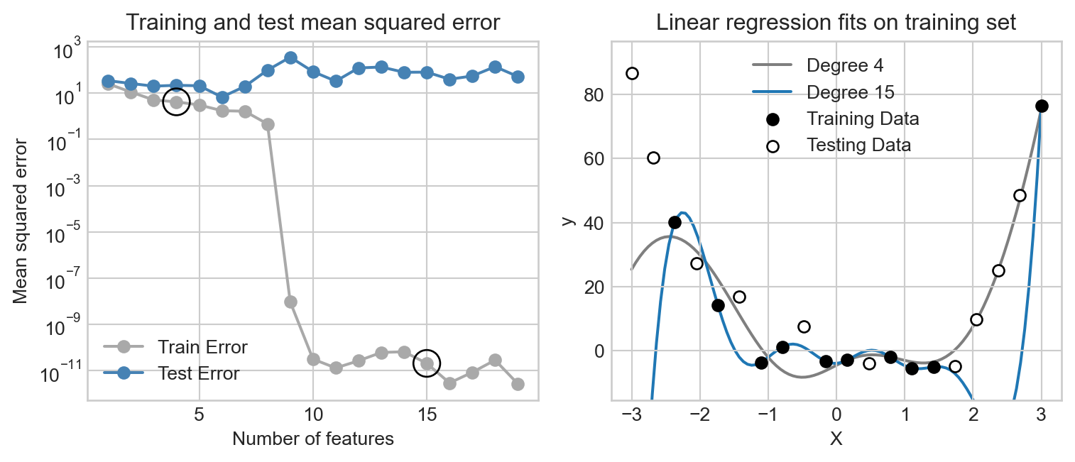
For a long time, pictures like this served as proof that interpolating the data is a bad thing to do and that therefore it is necessary to limit the number of parameters used when training models. The rise of deep learning, however, has challenged this viewpoint. Deep learning models are clearly stunningly successful, but often operate with massive numbers of parameters – these days on the orders of hundreds of billions (\(10^11\)). How could this be? In this blog post, you’ll implement a novel linear regression algorithm and show that, on some tasks, increasing the number of parameters well into the regime that would usually have been considered dangerous for overfitting can actually lead to optimal model performance.
Part 0
The standard formula for the optimal weight vector in unregularized least-squares linear regression with feature matrix \(\mathbf{X}\) and target vector \(\mathbf{y}\) is
\[ \DeclareMathOperator{\argmin}{argmin} \]
\[ \begin{aligned} \hat{\mathbf{w}} &= \argmin_{\mathbf{w}} \lVert{\mathbf{X}\mathbf{w} - \mathbf{y}}\rVert^2\;, \end{aligned} \]
which has closed-form solution
\[ \begin{aligned} \hat{\mathbf{w}} &= \left(\mathbf{X}^T\mathbf{X}\right)^{-1}\mathbf{X}^T \mathbf{y}\;. \end{aligned} \tag{1}\]
only when the number of data observations \(n\) is larger than the number of features \(p\). Please explain exactly what goes wrong in Equation 1 if \(p\) is instead larger than \(n\). In particular, which mathematical operation in Equation 1 is not allowed, and why?
Part A: Implement Overparameterized Linear Regression
If you have already implemented LinearModel from previous warmups and blog posts with a score method, all you need to do for this part is:
First, implement a MyLinearRegression model which inherits from LinearModel. This class only needs to implement MyLinearRegression.predict(X) (which simply returns the score) and MyLinearRegression.loss(X,y), which computes the mean-squared error loss between the score and the targets y.
Second, implement an OverParameterizedLinearRegressionOptimizer. This class should have a fit(X,y) method which computes the optimal weights for the model. In this problem, we’ll use the formula
\[ \begin{aligned} \hat{\mathbf{w}} &= \mathbf{X}^+ \mathbf{y} \\ \end{aligned} \]
where \(\mathbf{X}^+\) is the Moore-Penrose pseudoinverse of \(\mathbf{X}\). In the overparameterized case, the formula for \(\mathbf{w}^*\) is \(\mathbf{X}^T (\mathbf{X} \mathbf{X}^T)^{-1}\); however, rather than implementing this formula you can instead use the function torch.linalg.pinv(X) to compute the pseudoinverse.
This formula for \(\mathbf{w}\) comes from analytically solving the problem \(\hat{\mathbf{w}} = \argmin_{\mathbf{w}} \lVert{\mathbf{w}}\rVert\) subject to the requirement that \(\mathbf{w}\) leads to perfect interpolation: \(\mathbf{X}\mathbf{w} = \mathbf{y}\).
You should be able to use your model like this, on either X_train itself or a feature matrix generated from RandomFeatures.
LR = MyLinearRegression()
opt = OverParameterizedLinearRegressionOptimizer(LR)
opt.fit(X_train, y_train)
# now LR.w has the optimal weight vector
Part B: Test Your Model on Simple Data
Once you’ve implemented the model above, try using it to fit a model to some 1-d data:
X = torch.tensor(np.linspace(-3, 3, 100).reshape(-1, 1), dtype = torch.float64)
y = X**4 - 4*X + torch.normal(0, 5, size=X.shape)

plt.scatter(X, y, color='darkgrey', label='Data')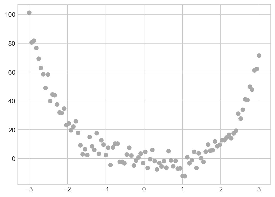
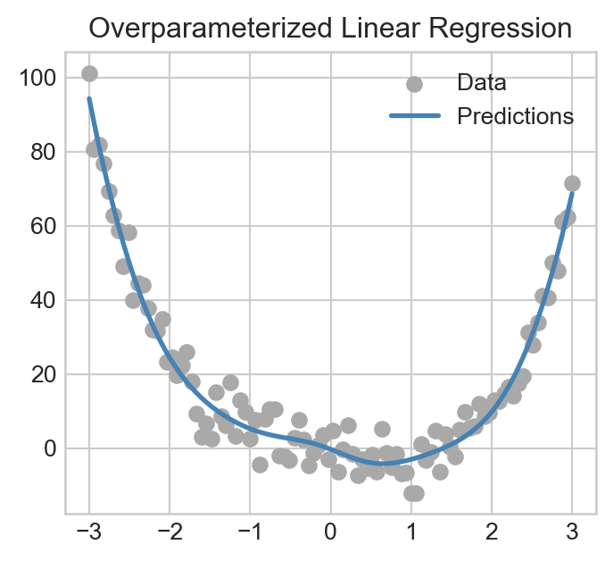
To fit a model to this nonlinear data set, you should first use the RandomFeatures class to generate a set of features which you then feed into your custom MyLinearRegression model. You should then plot the model predictions alongside the data, like this:
We’re not worrying about a train-test split here because we’re just checking that your model does something reasonable – think of this as a check that you can use to debug.
Part C: Double Descent In Image Corruption Detection
Now you’ll apply your model to a more complicated data set. Here’s our scenario: we have the following greyscale image of a beautiful flower:
from sklearn.datasets import load_sample_images
from scipy.ndimage import zoom

dataset = load_sample_images()
X = dataset.images[1]
X = zoom(X,.2) #decimate resolution
X = X.sum(axis = 2)
X = X.max() - X
X = X / X.max()
flower = torch.tensor(X, dtype = torch.float64)

fig, ax = plt.subplots(1, 1, figsize=(6, 6))
ax.imshow(flower)
off = ax.axis("off")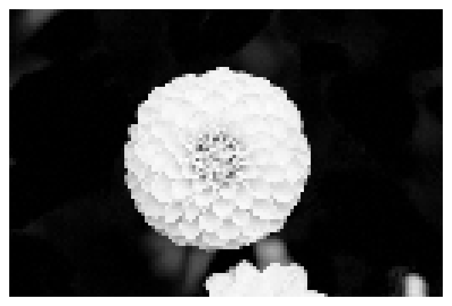
However, this image has some variable amount of corruption represented by contiguous blocks of grey pixels, which is implemented by the following function. This function adds a random number of randomly-sized grey patches to the image, and also returns the number of patches added.
def corrupted_image(im, mean_patches = 5):
    n_pixels = im.size()
    num_pixels_to_corrupt = torch.round(mean_patches*torch.rand(1))
    num_added = 0

    X = im.clone()

    for _ in torch.arange(num_pixels_to_corrupt.item()):

        try:
            x = torch.randint(0, n_pixels[0], (2,))

            x = torch.randint(0, n_pixels[0], (1,))
            y = torch.randint(0, n_pixels[1], (1,))

            s = torch.randint(5, 10, (1,))

            patch = torch.zeros((s.item(), s.item()), dtype = torch.float64) + 0.5

            # place patch in base image X
            X[x:x+s.item(), y:y+s.item()] = patch
            num_added += 1


        except:
            pass

    return X, num_added
We can use it like this:
X, y = corrupted_image(flower, mean_patches = 50)
fig, ax = plt.subplots(1, 1, figsize=(6, 6))
ax.imshow(X.numpy(), vmin = 0, vmax = 1)
ax.set(title = f"Corrupted Image: {y} patches")
off = plt.gca().axis("off")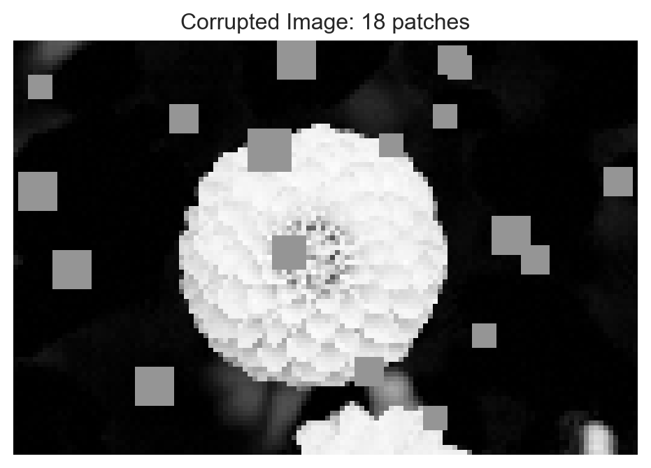
Our regression task is to predict the number of corruptions in the image just from the image itself. To do this, we’ll generate a data set of corrupted images.
n_samples = 200

X = torch.zeros((n_samples, flower.size()[0], flower.size()[1]), dtype = torch.float64)
y = torch.zeros(n_samples, dtype = torch.float64)
for i in range(n_samples):
    X[i], y[i] = corrupted_image(flower, mean_patches = 100)
Now we’ll reshape the image (laying its pixels out it one long row) and split the data into training and test sets.
X = X.reshape(n_samples, -1)
# X.reshape(n_samples, -1).size()

X_train, X_test, y_train, y_test = train_test_split(X, y, test_size=0.5, random_state=42)
Your Task
Please assess the performance of your model on this data set as you vary the number of features used by the RandomFeatures class (i.e. tune n_features). For this problem, I found it helpful to use a squaring activation for my feature map instead of a sigmoid activation, which corresponds to \(\phi(\mathbf{x}) = (\langle \omega_j, \mathbf{x}\rangle + b)^2\); you can do this by constructing your feature maps with phi = RandomFeatures(n_features = n_features, activation = square). For each choice of n_features, plot the training and test mean-squared errors. Please also plot a vertical line at the interpolation threshold, (the point at which the number of features used exceeds the number of training samples).
I found it useful to plot my training and test MSEs on logarithmic scale.
Your final result should look something like this:
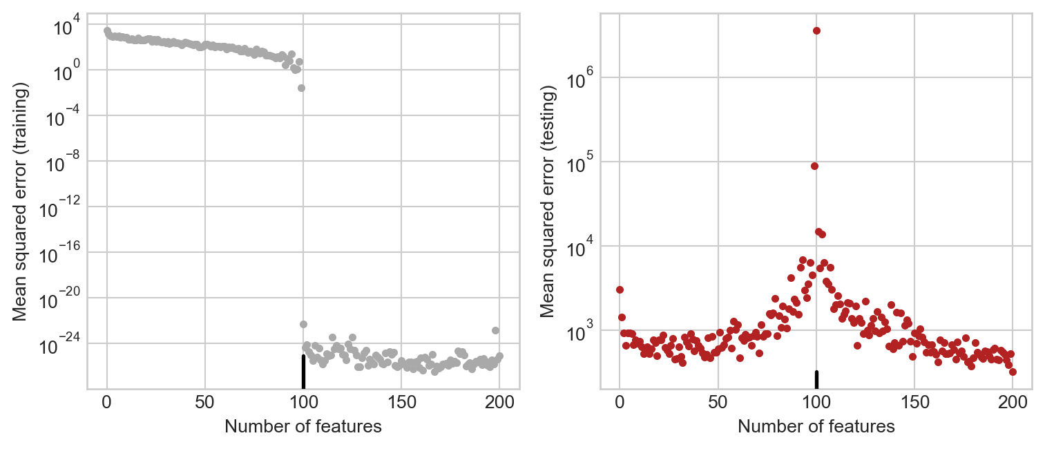
Finally, state the number of features at which you achieved the best testing error. Was the optimal number of features below or above the interpolation threshold?
Note: The plot on the righthand side shows the phenomenon of double descent: as we increase the number of features, the test error decreases, then increases as we approach the interpolation threshold, and then decreases again past the interpolation threshold. Many large models exhibit the phenomenon of double-descent.
Part D: Abstract and Discussion
Please add an introductory “abstract” section to your blog post describing the high-level aims of of your analysis and an overview of your findings. The abstract should be no more than one paragraph. Then, add a closing “discussion” section of your blog post in which you summarize your findings and describe what you learned from the process of completing this post.
Part E (Nothing to Submit): Why Does This Work?
The short explanation for the phenomenon of double-descent is that interpolating the data is not always bad: sometimes interpolating the data can actually lead to very reasonable-looking models. Here’s an example: simple “connecting the dots” in this model (linear interpolation) leads to a model that does better than the fancy feature maps at predicting unseen test data:
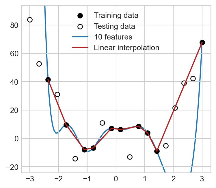
It is widely thought that a more complicated version of this phenomenon is partially responsible for the success of overparameterized deep neural networks.
© Phil Chodrow, 2025