Complexity0. Learning objectives
So far, we've written solutions to computational problems, but we haven't studied how efficient these solutions are. As we've seen several times, there is usually more than one way to solve a problem. The main question we want to think about today is how much computational resources will we need for a particular solution to a problem? These resources could include computational time and also memory. Although memory is a relevant constraint, we are quite sensitive to the time it takes for an algorithm to complete the computation it was designed to complete! More specifically, how does this time grow with respect to the size of the problem (e.g., Let's say that I design an new algorithm to sort a list of N values. If I double N, how is the time it takes my new algorithm to sort the list going to be affect? Will it change at all? If it does, will it change in a linear - $n$, logarithmic - $\log(n)$, polynomial - $n^k$, exponential - $a^n$, or factorial - $n!$ - way?). This is the study of computational complexity. |
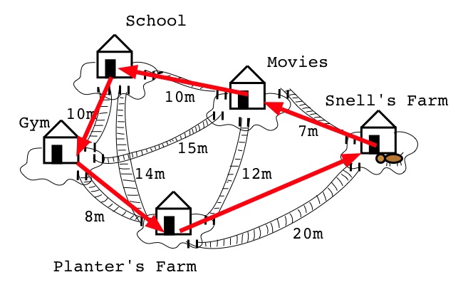 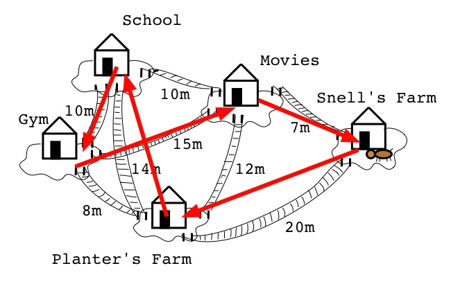 Two possible solutions to the traveling salesperson problem. (source) |
Consider the example to the right. This is a solution to the traveling salesperson problem (TSP) which asks: "given a list of cities and distances between cities, what is the shortest possible path that visits all cities exactly once and returns to the starting city." This is an example of a hard problem. With this we mean that, despite the fact that we can write code to find the optimal solution of the problem, the complexity (number of steps necessary to find the solution, hence time it would take to find the solution) is so high that for all intent and purposes, it is impractical to use. For this particular case, in order to answer the question with the optimal solution, we would need to go through every possible combination of starting points and paths. We have $n$ options to start with. Once we pick the starting point, we have $(n - 1)$ option for the second city, $(n - 2)$ for the thirds and so on, arriving at a whooping $n\cdot(n - 1)\cdot(n - 2)\cdots3\cdot2\cdot1$ possible paths to evaluate. This brute-force solution can be computed in $n!$ time ($\mathcal{O}(n!)$), which makes it pretty much pointless. Imagine that, assuming that you have a system that can evaluate 1 billion paths every second, it would take your system 77.1 years to find the optimal solution for just 20 cities, and 8400 trillion years for 30!!! (the universe is around 14 billion years old).
So, how do we evaluate the optimal path to deliver packages? How does your GPS give you the optimal route from point A to point B in definitely less than 77 years? We developed heuristic algorithms which, although they are not guaranteed to give you the optimal solution, they often can give you a reasonable solution in a reasonable time. Think of them as informed guesses. So, for example, we could use a greedy algorithm to solve TSP: we pick a random starting point and then we choose the least expensive route to the next point and so on. It might not give you the optimal solution but, if all the distances are reasonable, you will get a reasonable solution. Other examples are the Dijkstra's algorithm or the A* search algorithm to find the shortest path between two points.
The study of computational complexity also asks which problems can be actually be solved with a computer (computability). For example it answer question such as "can every problem be solved computationally?"... and the answer is... NO! (Take a look at the famous halting problem - watch also this for a cool animation about it).
1. Big-oh notation
In order to study the complexity of an algorithm, we need a of way of measuring the performance (whether that be run time or memory). Further, we want to estimate the performance of an algorithm when the inputs get really really really BIG. This is done using big-oh notation, which is represented by a "big O": $\mathcal{O}$.
Big-oh notation is a useful way to characterize how a function grows without caring too much about the details of the function. You can think it of a way to quickly represent how many "steps" an algorithm has to take in order to solve a problem of a given size $n$. "Size" should be interpreted a little loosely. It could be the actual number of elements in a list or it could be the $n$-th element in a progression that we want to compute (think Fibonacci). For example, if we think about the time that it will take for an algorithm to run, what we might want to know is: does an algorithm run in linear time (denoted by $\mathcal{O}(n)$)? or does it run in quadratic time (denoted by $\mathcal{O}(n^2)$)? or does it run in factorial time (denoted by $\mathcal{O}(n!)$)? or maybe it runs in constant time ($\mathcal{O}(1)$) where the computation time does not depend on the size of the problem at all!
|
We don't really care about whether it runs in $\mathcal{O}(2n)$ or $\mathcal{O}(3n)$ - we simplify that to just be linear time, $\mathcal{O}(n)$. Despite $3n$ being worse than $2n$, for the characterization of complexity, we don't care about the $2$ or the $3$ because these are constant factors on the function inside the $\mathcal{O}$. Ultimately, we're interested in placing an upper bound on the performance, so that we know our algorithm will always perform better than this upper bound. When designing an algorithm, we would like the stuff inside the $\mathcal{O}$ to not grow, or grow as slowly as possible. So we would prefer an algorithm that runs in $\mathcal{O}(n)$ time instead of an algorithm that runs in $\mathcal{O}(n^2)$ time; similarly we would prefer an algorithm that runs in in $O(n\log n)$ instead of an algorithms that runs in $\mathcal{O}(n^2)$... and forget about $\mathcal{O}(n!)$ that will literally take forever for very small values of $n$. |
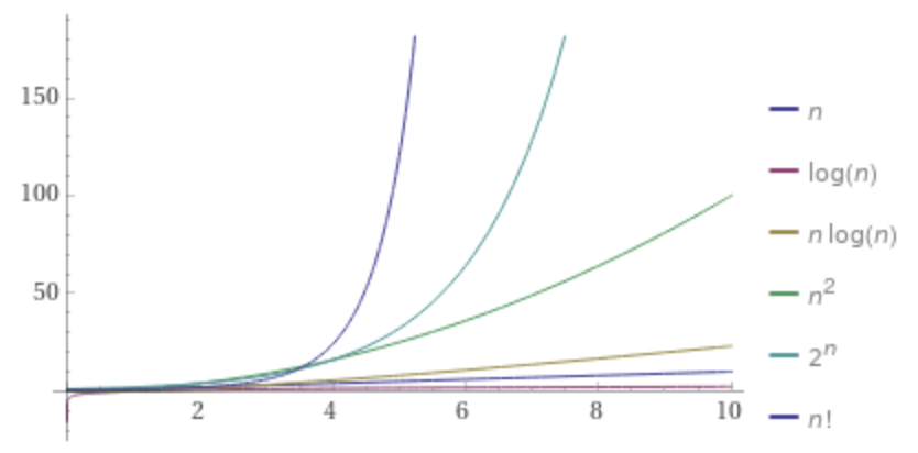 Growth of the different function with respect to their parameter $n$. You can think of $n$ as the size of the problem and the vertical axis as, for example, the time will take an algorithm with that complexity to solve the problem (faster is often better)! |
Example: Fibonacci
Consider, for example, the following algorithms (some of which we have seen before) that can be use to solve the same problem: calculate the $n$-th element in the Fibonacci sequence. Before you run the code, take a look and think about the algorithms. Which one do you think is going to take longer? If we consider $n$ the size of the problem, what do you think is the relationship between $n$ and the time (number of steps) the different algorithms need to perform to solve the problem (return the $n$-th element of the series)?
Once you run the code (my suggestion is to download it and run it in Thonny), you can change the value of $n$ at the top and look at the different timings. Here is a fun experiment (in Thonny). Start with $n$ = 30, run the code and annotate the times it takes for the 3 algorithms in a table. Then increase to 31, 32, up to 35, 36 (I wouldn't go much higher). Can you see a relationship? (You might want to run it a couple of times for each value of $n$ and take an average to get a better measurement.
The recursive approach has a complexity of $\mathcal{O}(2^n)$. Each time you increase $n$ by one, the time that it takes to compute the solution doubles! This is an example of a hard problem. As a matter of fact, we consider any problem that has a complexity that can be expressed as $\mathcal{O}(n^k)$ (polynomial) to be an easy problem. As you can see, hard has no bearing on how hard is to write the code that solves the problem. Probably the recursive Fibonacci is the simplest code in this example but, computationally, the number of steps required increases exponentially making it a hard problem.
The imperative approach has a complexity of $\mathcal{O}(n)$. If you look at it, you can see that there is a loop that will iterate about $n$ times in order to solve our problem. This means that if I double $n$, it will probably take twice as long. We say that the problem is linear in time.
Finally, using the Binet's formula to calculate the $n$-th element of the Fibonacci series always takes the same time and, its complexity can be represented as $\mathcal{O}(1)$, independent from $n$. We also call this constant time.
1.1. Best, worst and average case analysis
So how do we go from an algorithm to estimating the performance?
Well, maybe we can write up the algorithm (into actual code) and then just run some experiments to estimate how long it takes to run for various input sizes. This isn't the most practical approach because you might end up waiting a long time for your program to run. Instead, we can look at the pseudocode to try to count the the number of operations performed.
We previously talked about how computers perform operations at a particular rate (GHz), i.e. the number of
operations per second. The total time spent on an algorithm is, therefore, dependent on how many operations are
performed. In the examples on searching and sorting below, we will focus on counting the number of
comparisons performed, using comparative operators like == or <.
When counting operations, we might want to consider how many operations are performed in the best case, worst case or average case. (Analyzing the average case requires some probability theory, so we won't do that in our course). Just as it sounds, a best case analysis is one the treats the best possible case (for the inputs) to our algorithm. For example, in a sorting algorithm, this algorithm might perform really well if the input list is already sorted. A worst case analysis involves being really pessimistic about the inputs to your algorithm (hence, being the worst case). In other words, you want to assume that any comparison that might be made will be made. For example, in a sorting algorithm, if we want to sort the list from smallest to biggest, but the input list is sorted from biggest to smallest, then this might be the worst case for the algorithm (again, best and worse case will depend on the task at hand).
1.2. Divide-and-conquer algorithms
Before we see some specific algorithms for searching and sorting, let's introduce the idea of a divide-and-conquer algorithm.
These are algorithms that break up the current problem into smaller pieces (the divide stage), assuming that we can eventually reach some base case which we know how to solve. Then we can conquer our original problem by using the solution to the smaller problems. If this sounds pretty recursive, doesn't it? This is because divide-and-conquer algorithms are often implemented using recursion!
2. Searching algorithms
In a searching algorithm, the goal is to identify whether a list contains a specific value. In the case of numbers, for example, there are two inputs: some number we are looking for and a list of numbers. The size of the list gives the size of the problem, the "$n$". What we care about when analyzing the performance (computational complexity) of a searching algorithm is how "long" it will take with respect to $n$.
2.1. Linear search
A naive approach would be to go through every item in the list, starting from the beginning and check, using
==, whether the item in the list matches the value we are looking for. In the best case, the
item we are looking for is in the first item in the list, so only 1 operation is needed: $\mathcal{O}(1)$. In
the worst case, the item we are looking for is at the end of the list, so $n$ operations are required:
$\mathcal{O}(n)$. As before, change the code and try different values of $n$ and see if you can notice a
relationship between the time it takes and the value of $n$. Are the values stable for a given $n$? Do they
change a lot? Why do you think that is the case? How would you provide a measure of the time this algorithm
takes as function of $n$?
2.2. Binary search
We can actually do much better in our searching algorithm by employing a divide-and-conquer approach. This particular algorithm will only work if we can assume that the input list is sorted! If it is, then we can run our algorithm recursively each time halving the input list and looking in only one of the halves.
How does it work? Because of our assumption about the list being sorted, checking the middle of the list will tell us which half of the list we can ignore. Then, for the half we are not ignoring, we can repeat the check in the middle, and so on. This saves a lot of computation! In the best case, we might still find the value in the first item in the list: $\mathcal{O}(1)$. In the worst case, we will need to perform $\mathcal{O}(\log_2 n)$ operations. Don't worry how to derive this for now - but take CS 200 if you're interested in learning more. Ultimately the $\log_2 n$ comes from asking "how many times do we need to break a list in half until we get to a sublist of length 1 (the base case)?"
Try to mess with the size of the problem and compare the timing of the two algorithms.
3. Sorting algorithms
In binary search, we made an assumption that the input list was already sorted - but how do we sort the items in a list? In sorting algorithms, our only input will be a list, and the "$n$" will be the length of the list (the number of items). Our goal is to sort the input list from the smallest to the largest item.
3.1. Selection sort
|
A naive approach to sorting items in a list consists of starting from the first item, go through the entire list looking for the smallest item and, once we have went through the entire list, replace the first item with the smallest one. Then start from the second item, and repeat the process. Then the third, the fourth, and so on until we have repeated the process for all the items in the list. (An illustration of the selection sort algorithm is shown on the right. Yellow items are already sorted. Red items show the current minimum in the scan through the remaining list. Items currently being scanned are shown in blue. When an arrow appears, the two items on either side of the arrow are swapped). In more detail, you can imagine a scanning line that moves from left to right (or top to bottom in the diagram on the right) through the items in the list. The first time this scanning line passes through the list, it starts at item 1 and then traverses the entire list to search for the smallest item. When it finds it, this smallest item will be placed at the beginning of the list (index 0). Index 0 now contains the smallest item, so it doesn't make sense for our scanning line to start there - we will now start scanning at index 1 and search for the second smallest item. This second smallest item will then be placed at index 1 of the list. Scanning then starts at index 2 and scans for the third smallest item, and so on, iteratively looking for the smallest remaining item in the list. |
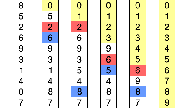 (source) |
|
|
So, if we start scanning at index 0 and we go to the end of the list, how many comparisons
( |
3.2. Insertion sort
|
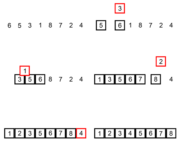
Another sorting algorithm which has a better performance than selection sort is insertion sort. This mimics the way you would probably sort cards in your hand. In this case, the sorting is still done in place, by iterating over the list. Once again you can imagine the sorted part of the list to the left and the unsorted to the right of an imaginary line. As the line moves to the right, each unsorted item is picked in turn and moved to the sorted part of the list to the left as long as the item to its left is larger. In other words, the first unsorted item is picked up from the unsorted part of the list and moved to the left until it can be inserted in the correct position within the sorted part of the list. |
 |
|
|
In comparison to selection sort, this algorithm will perform differently if presented with an already
sorted list (best case) or a list sorted backward (worse case). In the worse case scenario the algorithm
will also run in $\mathcal{O}(n^2)$, just like selection sort. The advantage is that, when presented with
the best case scenario, the runtime is reduced to $\mathcal{O}(n)$. If you look at the code below, you
will notice that the inner loop (the one that places the item in the correct position within the sorted
part of the list, is obtained using a As you look at the code, imagine calling the function with an already sorted list and a list that is sorted backward and ask yourself how the while loop behaves in these scenarios. |
3.3. Merge sort
Can we do better than $\mathcal{O}(n^2)$ for sorting a list of numbers? Yes, in fact, we can use a divide-and-conquer approach to recursively sort two halves of the input list (dividing our original problem into two smaller sub-problems) and then merge the two sorted sublists. The merge sort algorithm has a run time of $\mathcal{O}(n\log_2 n)$ which is slower than $\mathcal{O}(n)$, but faster than $\mathcal{O}(n^2)$.
Let's illustrate the basic idea of merge sort:
- Check if the input list has a length less than 2. If so, a list with 1 (or no) item is already sorted!
- Otherwise, split the input list into two halves: a left sublist and a right sublist,
- Sort the left and right sublists recursively (i.e. calling
merge_sort) on these two sublists, - Merge the resulting sorted sublists into the a sorted length $n$ list.
|
|
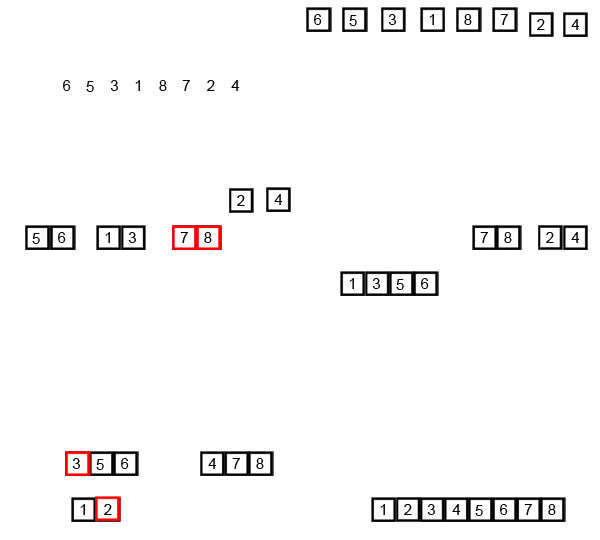 Illustration of the merge sort algorithm. Items in red are those that are currently being compared during the merge stage. (source). |
In merge_sort, all comparisons (<) are done in the "merging" stage. It can be shown
that, in the worst case, merging two sublists of length $n/2$ requires $n-1$ operations (about $n$). Since we
need to divide our original list $\log_2(n)$ times to get to our base case, this leads to the result that merge
sort requires, in the worst case, $\mathcal{O}(n\log_2 n)$ operations to sort a list of length $n$.
Here is the algorithm in all his glory: