Welcome to CSCI 0451: Machine Learning!
Spring 2026
Prof. Phil Chodrow
Department of Computer Science
Middlebury College
Hi everyone!
I’m Prof. Phil Chodrow. Please call me “Phil” or “Prof. Phil.” “Prof. Chodrow” is ok if that’s what makes you comfortable.
I think about….
Math, social networks, applied statistics, information theory, effective teaching
I like…
♟️ Chess (let’s play!), 🎿 nordic skiing, 🍵 tea, 🍵 hiking, 🥘 cooking, 📖 reading, 🖖🏻 Star Trek Deep: Space Nine.
Two fun facts
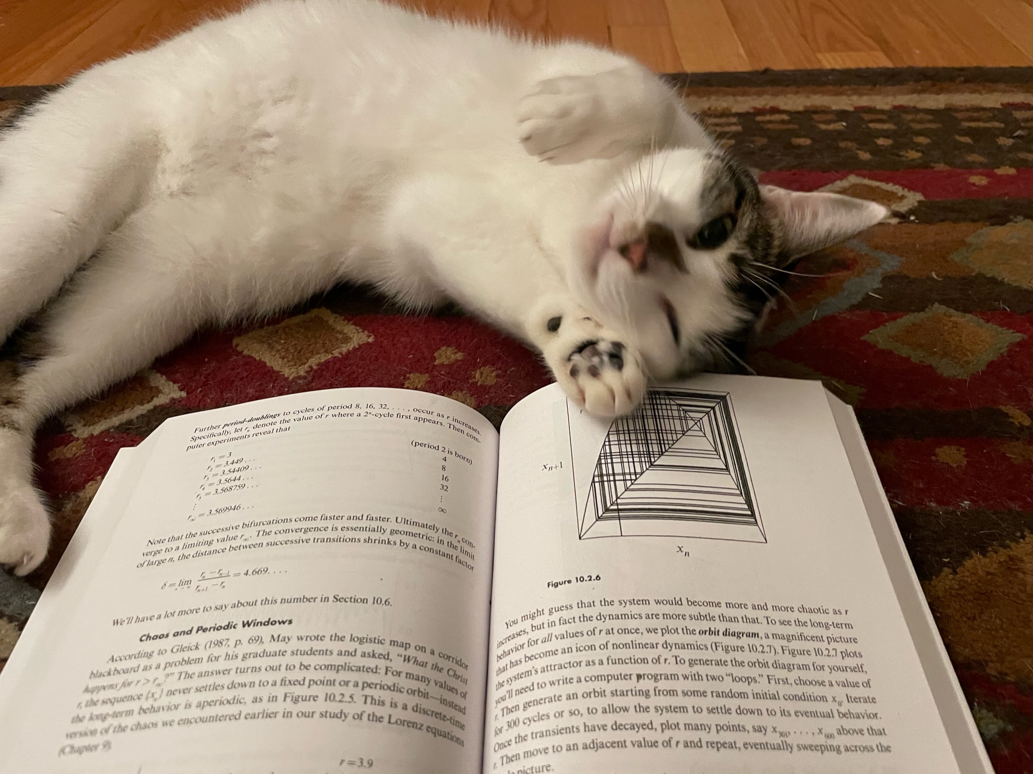
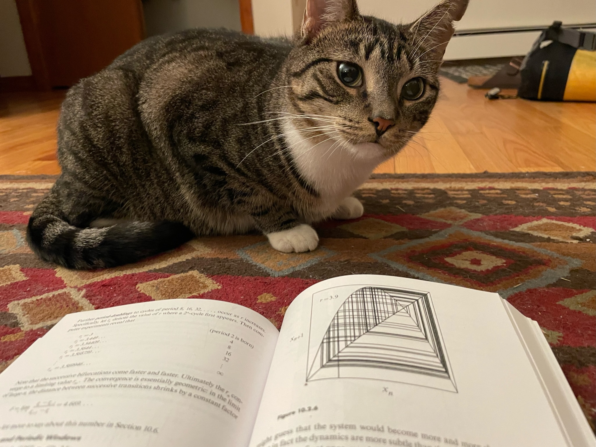
I have two cats who also love math
![]()
![]()
I practice aikido (and had short hair)
![]()
Today
- What is machine learning and why should we study it?
- What are we going to learn in this course?
- How will we learn and demonstrate our learning?
- Introducing Data = Signal + Noise
Your Affinity Vegetable
1. Split into teams
2. Go around and share your name and:
If you were a vegetable, which vegetable would you be and why?
Hello! My name is Phil and if I were a vegetable, I would be garlic. Garlic can be either a quiet helper or a charismatic center of a dish, and that reflects my personality as part introvert and part performer.
Your Affinity Vegetable
3. As a group identify a delicious dish that incorporates all of your vegetables.
Be ready to share!
Today
- What is machine learning and why should we study it?
- What are we going to learn in this course?
- How will we learn and demonstrate our learning?
- Introducing Data = Signal + Noise
Machine learning is…
…the theory and practice…
…of designing automated systems for prediction and decision-making…
…which adapt their behavior based on data.
Machine learning is the theory and practice of designing automated systems for prediction and decision-making which adapt their behavior based on data.
- Amazon makes recommendations for things you might want to buy based on your browsing and purchase history.
- TikTok curates your feed based on your previous interactions and searches.
- GPT/Copilot/Gemini/Claude generate text, code, images, and music in response to your prompts after training on huge internet corpora.
How many times have you interacted with an automatic recommendation, a personalized ad, a curated feed, or a generative AI model since you woke up today?
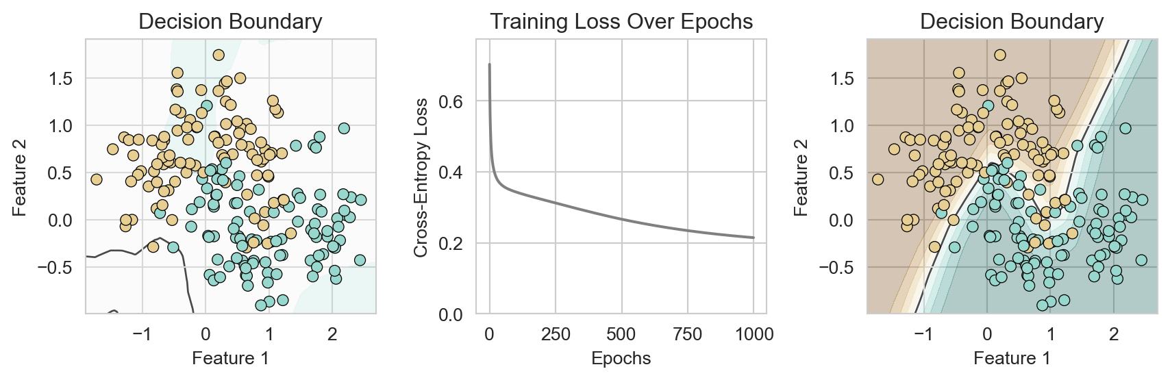
Example: Learning to Classify
As technical specialists, we’ll be especially interested in understanding what is happening in the training process and how to measure how well it worked.
Today
- What is machine learning and why should we study it?
- What are we going to learn in this course?
- How will we learn and demonstrate our learning?
- Introducing Data = Signal + Noise
A common ML course
- Introduction to machine learning and the Python ecosystem (weeks 1-2)
- Regression
- Logistic regression
- Support vector machine
- Decision trees and random forests
- Deep learning
- …
By the end of the course: you know a little bit about a lot of methods and can use them in applications.
What we are doing here
- Theoretical frameworks for machine learning: data = signal + noise.
- Regression and classification as instances of this theoretical framework.
- Math + computational techniques for actually fitting models.
- Deep learning as an extension of these ideas.
By the end of the course: you will be the smartest person in the room about the algorithmic structure of modern machine learning algorithms.
Learning objectives
Theory: math of models and training.
Experimentation: evaluating the performance of models on real and synthetic data
Social Responsibility: thinking critically about the social impacts of the models we build.
Implementation: creating models in structured code.
Navigation: working with the Python ecosystem, especially pytorch.
Why so much theory?
The future of machine learning belongs to those who understand why models work, how to evaluate them, and when to use them.
This includes:
\[
\begin{aligned}
f(\mathbf{x}; \mathbf{w}) &= \sigma(\mathbf{w}^\top \mathbf{x}) &\text{(model)} \\
\ell(y_i, s) &= - \left[ y_i \log(s) + (1 - y_i) \log(1 - s) \right] &\text{(loss function)}\\
L(\mathbf{w}) &= \sum_{i=1}^n \ell(y_i, f(\mathbf{x}_i; \mathbf{w})) \\
\nabla_{\mathbf{w}} L(\mathbf{w}) &= \sum_{i=1}^n (f(\mathbf{x}_i; \mathbf{w}) - y_i) \mathbf{x}_i &\text{(gradient)} \\
\mathbf{w}' &\leftarrow \mathbf{w} - \eta \nabla_{\mathbf{w}} L(\mathbf{w}) &\text{(training loop)} \\
\end{aligned}
\]
Today
- What is machine learning and why should we study it?
- What are we going to learn in this course?
- How will we learn and demonstrate our learning?
- Introducing Data = Signal + Noise
A Typical Class Day
Before
|
Complete the warmup problem ahead of class and submit on Gradescope
|
During
|
Present the warmup problem to your group (~15 mins).
Lecture: theory (~25 mins) + implementation and experiments (~25 mins).
|
After
|
Work on the week’s homework assignment or miniproject.
Study lecture notes to prep for quizzes and exam.
|
Formative assessments are for you to deepen your understanding outside of class.
Homework assignments (roughly 5)
- Problems for practicing concepts from lecture.
- Will often involve math (differential calculus, linear algebra)
- Prepare for quizzes and exams
- Opportunity for revision if submitted by first due date.
- Warmup problem is graded on effort and counts towards homework grade.
Mini-projects (roughly 4)
- Open-ended implementation and experimentation projects.
- Mostly coding and writing in Jupyter notebooks
- (Optional): post your miniprojects on an online portfolio.
Summative Assessments
Summative assessments are to hold you accountable to good learning practices and evaluate your growth in the material.
Timed Assessments
- Quizzes (in class, roughly 3)
- Midterm exam
- Oral exam
Closed book, timed, proctored assessments that draw on a similar problem bank as the homework.
Project
A ~4 week long project in which you apply methods from class to a project of your choice, completed as a group.
Generative AI
Generative AI can inhibit learning new code (Shen and Tamkin 2026) and math (Bastani et al. 2025), even when it is making you feel like you are learning and achieving more (Becker et al. 2025).
We find that AI use impairs conceptual understanding, code reading, and debugging abilities, without delivering significant efficiency gains on average.
(Shen and Tamkin 2026 on experienced coders learning a new library):
Generative AI Policy: You’re an Adult
50% of your course grade comes from quizzes, the midterm, and the oral exam. These are timed, proctored assessments without access to external resources.
The purpose of the homework and warmup is to help you practice for these assessments.
You’ll get the most out of that practice if you do it without AI assistance, especially the math.
Use of generative AI for coding in homework, miniprojects, and the final project is likely to be helpful in moderation but may also lead to headaches. I’ll just ask you to note in a statement when you use generative AI and what you used it for.
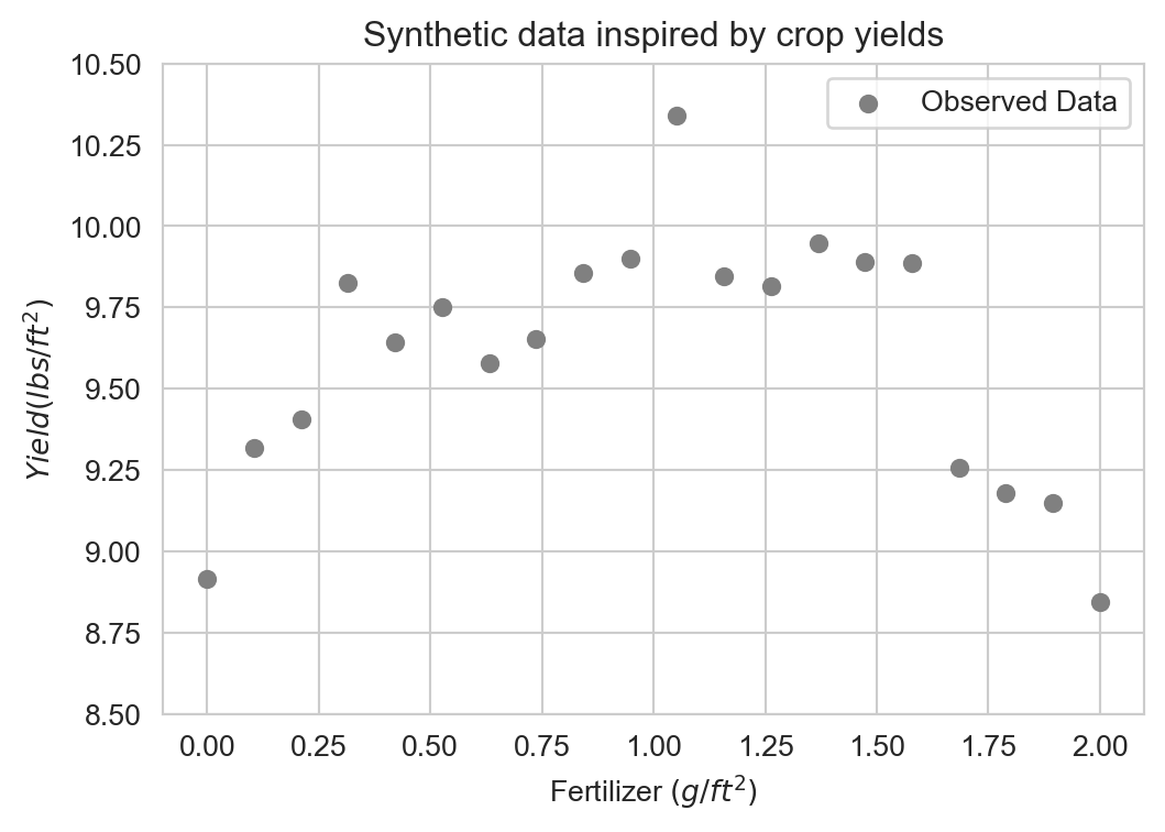
Onward: First Steps Towards Modeling
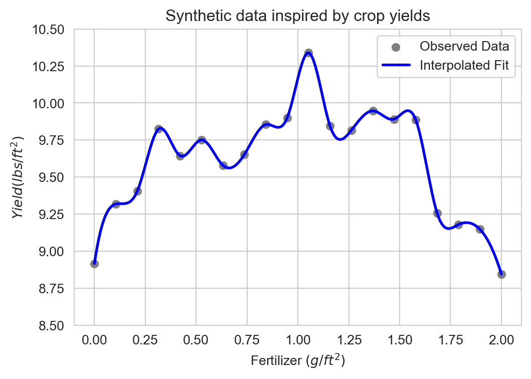
Suppose we have the following data set which we’d like to model:
Interpolation
Perfectly fitting the data is called interpolation:
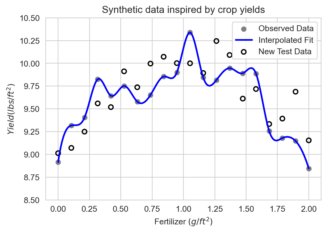
Interpolation often fails to generalize
This model performs poorly on similar new data:
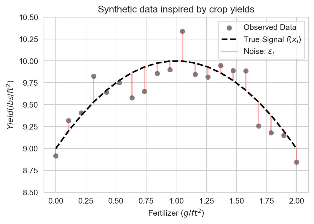
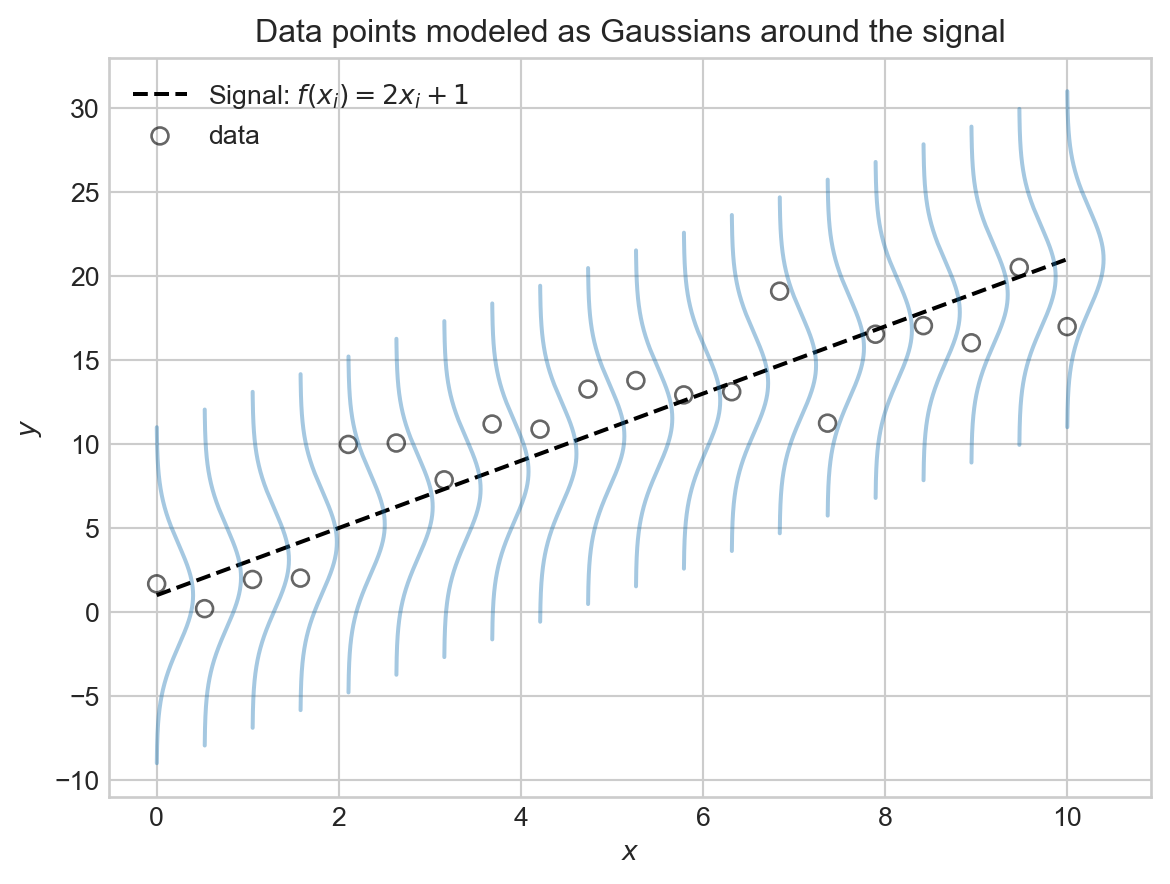
Data = Signal + Noise
A theoretical, schematic view of the data:
\[
\begin{aligned}
y_i = f(x_i) + \epsilon_i
\end{aligned}
\]
Successful machine learning modeling learns the signal \(f(x_i)\) while ignoring the noise \(\epsilon_i\).
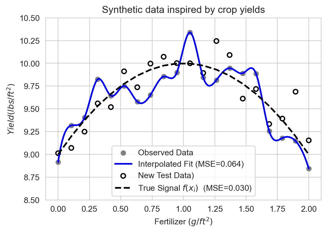
Data = Signal + Noise
Learning the true signal allows us to generalize better to new data:
\[
\begin{aligned}
MSE = \frac{1}{n} \sum_{i=1}^n (y_{i,\mathrm{actual}} - \hat{y}_{i,\mathrm{prediction}})^2
\end{aligned}
\]
Lower MSE on test set \(\implies\) better predictive performance.
In ML, we want to approximate the true signal from observations of noisy data.
Coming up…
Modeling signal and noise with linear trends and Gaussian probability distributions.
![]()
\[
\begin{aligned}
p(\epsilon;\mu, \sigma^2) &= \frac{1}{\sigma \sqrt{2 \pi}} \exp\left( -\frac{(\epsilon - \mu)^2}{2 \sigma^2} \right)
\end{aligned}
\]
Before Wednesday
Join Campuswire
Read the syllabus and post questions on Campuswire.
Complete the warmup problem (go/cs-451) and submit on Gradescope.
Email me LOAs