Miniproject: Count Regression with the Negative Binomial Distribution
In this miniproject, we’ll implement a custom kind of linear regression model for working with targets \(y\) that represent counts. Some examples of count data include:
Daily number of visitors to a website, store, or class.
Number of animals observed in a given area (abundance).
Number of times a certain event occurs (e.g. number of times a person visits the doctor in a year).
Count data is often unsuitable for the linear-Gaussian model (and therefore for least-squares linear regression) because it violates some major assumptions:
The linear-Gaussian model can generate negative target values \(y\), which doesn’t make sense for count data.
The linear-Gaussian model can predict non-integer target values, which also doesn’t make sense for count data.
In this miniproject, we’ll implement negative binomial regression, a kind of linear regression which is suitable for count data.
Negative Binomial Regression
The Negative Binomial Distribution
The negative binomial distribution is a discrete probability distribution which describes a random nonnegative integer: perfect for counts! It has two parameters: a mean \(\mu\) and a dispersion parameter \(r\). The probability mass function of the negative binomial distribution is given by:
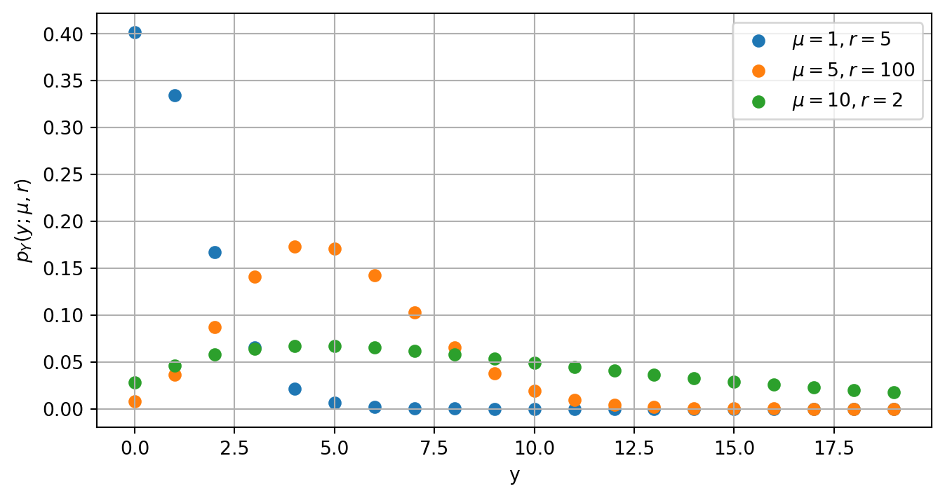
Here, \(\Gamma(z)\) is the gamma function. Here are some examples of the negative binomial distribution for different values of \(\mu\) and \(r\):
import torchimport matplotlib.pyplot as pltnbinom_pdf =lambda y, mu, r: (torch.lgamma(y + r) - torch.lgamma(r) - torch.lgamma(y +1) + r * torch.log(r) + y * torch.log(mu) - (y + r) * torch.log(r + mu)).exp()y = torch.arange(0, 20)mu_values = torch.tensor([1, 5, 10])r_values = torch.tensor([5, 100, 2])fig, ax = plt.subplots(figsize = (8, 4))for i inrange(3): mu = mu_values[i] r = r_values[i] pmf = nbinom_pdf(y, mu, r) ax.scatter(y, pmf, label=fr"$\mu={mu.item()}, r={r.item()}$")ax.grid()plt.xlabel("y")plt.ylabel(r"$p_Y(y; \mu, r)$")plt.legend()
Figure 1: Examples of the negative binomial distribution for different values of \(\mu\) and \(r\). The value of \(p_Y(y; \mu, r)\) is the probability that a random variable \(Y\) with a negative binomial distribution takes the value \(y\).
Regression Problem
In negative binomial regression, we assume that the target variable \(y\) follows a negative binomial distribution, where the mean \(\mu\) is given by the equations
The likelihood of a single data point \((\mathbf{x}_i, y_i)\) under the negative binomial regression model is given by plugging this expression for the mean into the negative binomial PMF:
where \(s_i = \mathbf{x}_i^\top \mathbf{w}\) and \(n\) is the number of data points in the dataset. To implement negative binomial regression, we can maximize this log-likelihood with respect to the parameters \(\mathbf{w}\) and \(r\) using gradient ascent. Alternatively, we can minimize\(\mathcal{L}(\mathbf{w}, r)\) and achieve the same outcome.
Data Set
Our data set for this miniproject is a data set of counts of cockroaches which was originally published by Gelman and Hill (2007). You can access the training data like this:
import pandas as pdurl ="https://middcs.github.io/csci-0451-s26/data/roaches/train.csv"train = pd.read_csv(url)train.head()
constant
y
roach1
treatment
senior
exposure2
0
1
15
53.00
1
0
1.0
1
1
1
91.88
1
1
1.0
2
1
0
2.00
1
1
1.0
3
1
24
5.44
0
0
1.0
4
1
50
42.00
1
0
1.0
Each row of this data set gives the number of cockroaches observed in a certain apartment in New York City at the time of data collection. Each observation includes:
The columns of the data include:
y, the target variable: the number of cockroaches observed by being found in traps.
constant, a column of 1’s which we can use to fit an intercept term.
roach1, the number of cockroaches observed in the previous survey of the same apartment.
treatment, whether or not the apartment was treated via an integrated pest management program.
exposure2, the number of trap-days used for data collection. A trap-day is one trap set for one day, so, for example, if 2 traps are set for 3 days then the exposure is 6 trap-days. For technical reasons related to negative binomial regression modeling, it is suggested to use the logarithm of this feature in modeling.
The following convenience function prepares the data and creates the feature matrix \(X\) and target vector \(y\) for training or evaluation:
def prep_data(df): df["exposure2_log"] = torch.log(torch.tensor(df["exposure2"].values, dtype=torch.float32)) df.drop(columns=["exposure2"], inplace=True) y = torch.tensor(df["y"].values, dtype=torch.float32) X = torch.tensor(df[["constant", "roach1", "treatment", "exposure2_log"]].values, dtype=torch.float32)return X, y
X_train, y_train = prep_data(train)
We’d like to train a negative binomial regression model on this data and then evaluate the model on a test set.
What You Should Do
0. Fire Up Google Colab
Please go to Google Colab and create a new notebook. You can name the notebook count_regression.ipynb. Save the notebook somewhere where you can find it.
If possible, I recommend connecting your Colab notebook to a GPU runtime. You can do this by going to the “Runtime” menu, selecting “Change runtime type”, and then selecting “GPU” as the hardware accelerator. This will allow you to train your model much faster than if you were using a CPU runtime.
1. Implement Negative Binomial Regression
To implement negative binomial regression, you’ll need to implement a model class, an optimizer, functions for the log-likelihood and loss, and a training loop.
Model Class
A NegativeBinomialRegression class. This class should:
Have an __init__ method that initializes the parameters \(\mathbf{w}\) and \(r\) as torch tensors with requires_grad=True. The __init__ method should take in the number of features as an argument and initialize \(\mathbf{w}\) to be a vector of zeros with the appropriate shape. You can initialize \(r\) to be any positive value (e.g. 1.0).
Have a forward method that takes in a matrix of features \(X\) and returns the vector of linear scores \(s = X \mathbf{w}\).
If you read this and think that this class sounds very similar to a standard linear regression model, you’re right! The only difference is that we have an extra parameter \(r\) for the dispersion of the negative binomial distribution.
Log-Likelihood and Loss Functions
A log_likelihood function that takes in a vector of scores \(\vs \in \mathbb{R}^n\), a vector of targets \(\mathbf{y}\in \mathbb{R}^n\), and the dispersion parameter \(r\), and computes the log-likelihood of the data under the negative binomial regression model. You should call your function log_likelihood(y, s, r).
A loss_fun function that takes in the parameters \(\mathbf{w}\) and \(r\), a matrix of features \(X\), and a vector of targets \(y\), and computes the negative log-likelihood of the data under the negative binomial regression model. I normalize the negative log-likelihood by the number of data points \(n\) to make it easier to interpret the loss values. You should call your function loss_fun(w, r, X, y).
Gradient Descent Optimizer
A GradientDescentOptimizer class that performs gradient descent to maximize the log-likelihood. This class should implement:
An __init__ method that takes in a model and a learning rate.
A step method that takes in a matrix of features \(X\) and a vector of targets \(y\), computes the gradients of the loss with respect to the parameters \(\mathbf{w}\) and \(r\), and updates the parameters using gradient descent with a fixed learning rate. You should compute the gradients using your grad_func method (described below) rather than using PyTorch’s autograd functionality.
A grad_func method that takes in the parameters \(\mathbf{w}\) and \(r\), a matrix of features \(X\), and a vector of targets \(y\), and computes the gradients of the log-likelihood with respect to \(\mathbf{w}\) and \(r\). You should compute these gradients by hand using calculus, and then implement the formulas in code.
Finally, you’ll need a training loop that creates an instance of your NegativeBinomialRegression model and your GradientDescentOptimizer, and runs gradient descent for a certain number of epochs.
Training Loop
You can train your model using a standard training loop in global scope. The main purpose of the training loop is to call the step method of your optimizer repeatedly to perform gradient descent. You can also print out the current value of the loss every so often to monitor training progress.
Implementation Notes
You can use torch.lgamma(y) to compute expressions like \(\log \Gamma(y)\), which appear in the log-likelihood.
The derivative of \(g(x) = \log \Gamma(x)\) is given by \(g'(x) = \psi(x)\), where \(\psi\) is the digamma function. You can compute \(\psi(x)\) using torch.digamma(x).
It’s hard to be confident that your formulas for the gradients are correct. It can help to check your work by comparing the output of grad_func to the output of PyTorch’s autograd functionality. You can do this by computing the loss using your loss_fun, calling loss.backward(), and then comparing the values of model.w.grad and model.r.grad to the output of your grad_func. Unfold the code cell below to see an example of how to make this comparison:
Code
model = NegativeBinomialRegression(num_features=X_train.shape[1])optimizer = GradientDescentOptimizer(model, lr=0.0001)# gradients from grad_funcgrad_w, grad_r = optimizer.grad_func(model.w, model.r, X_train, y_train)# gradients from autogradmodel.w.requires_grad_()model.r.requires_grad_()loss = loss_fun(model.w, model.r, X_train, y_train)loss.backward()# print the resultsprint("Gradient from grad_func:")print("w_grad:", grad_w)print("r_grad:", grad_r)print("\nGradient from autograd:")print("w_grad:", model.w.grad)print("r_grad:", model.r.grad)
2. Train Your Model
You can train your model simply by running the training loop you implemented in the previous part. To get a helpful sense of your model performance, I recommend withholding a portion of the training data (say, 30%) as a validation set, and then evaluating the log-likelihood of your model on the validation set every so often during training. You should see the log-likelihood on the validation set increase as training progresses.
Optional: Feature Engineering
You may wish to try adding additional features to your model, such as interaction terms (in which columns are multiplied together), polynomial features, or anything else you can think of. If you want to try this, implement a function with exact name add_features. add_features should accept the feature matrix X (a torch.Tensor) as input and return a new feature matrix with additional features added. You can call this function on the training data before training your model, and you can also call it on the test data before evaluating your model on the test set.
# example: adding an interaction term between roach1 and treatmentdef add_features(X): roach1 = X[:, 1] treatment = X[:, 2] interaction = roach1 * treatmentreturn torch.cat([X, interaction[:, None]], dim=1)
If you do add features prior to training your model, then you should make sure to evaluate your model on validation data in order to guard against overfitting.
3. Save Your Model
Save your model by pickling it to a file called model.pkl. You can do this using the pickle module in Python, which allows you to serialize and save Python objects. Here’s an example of how to save your model using pickle:
import pickle# ... training loopwithopen("model.pkl", "wb") as f: pickle.dump(model, f)
4. IMPORTANT: Restructure Your Notebook
To submit your work on Gradescope, we need to ensure that your notebook has a structure where the training loop won’t be run on the Gradescope server. For this reason, please restructure your notebook so that the training loop is inside an if __name__ == "__main__": block. This way, the training loop will only be run if you run the notebook yourself, and it won’t be run when Gradescope runs your notebook for evaluation.
Schematically, your notebook should look like the code block below. The code shown below should be distributed across multiple notebook cells, but should be in the order shown.
Note
Please restart your kernel and run all cells after making this change to ensure that your notebook still runs correctly!
import torchimport pandas import pickle# ...class NegativeBinomialRegression: # code for your model class# ...class GradientDescentOptimizer:# code for your optimizer class# ...def log_likelihood(y, s, r):# code to compute log-likelihood# ...def loss_fun(w, r, X, y):# code to compute loss# ...def add_features(X):# optional code to add features# ...# code to implement your model, optimizer, log-likelihood function, and loss function# optional implementation of add_features() function for feature engineeringif__name__=="__main__":# code to acquire and prep data X = add_features(X) # if you implemented add_features# code to train and save your model
5. Submit Your Work
To complete this assignment you must submit two things:
A Python script corresponding to your Colab notebook, with the training loop inside an if __name__ == "__main__": block as described above. You can convert your Colab notebook to a Python script by going to the “File” menu, selecting “Download”, and then selecting “Python (.py)”. Name this file count_regression.py and submit it on Gradescope.
A file called model.pkl which contains the pickled version of your trained model. You can create this file by running the cell in your Colab notebook which saves your model using pickle. Submit this file on Gradescope as well.
On Gradescope, your model will be evaluated on a test set of cockroach counts which is separate from the training data. Your model will be evaluated based on loss on the test set, where the loss is given by the negative log-likelihood of the test data under your model.
6. (Optional) Publish Your Notebook
Optionally, you may publish your notebook on a blog through GitHub Pages and Quarto. Follow the instructions here to publish your blog.
How You’ll Be Assessed
The autograder will check…
GradientDescentOptimizer.grad_func computes the same gradients of the parameters \(\mathbf{w}\) and \(r\) as PyTorch’s autograd functionality.
The loss of your model on the test set is below 3.6 (remember, that’s the negative log-likelihood divided by the number of data points in the test set).
The grader will check…
Your code is well-organized and makes good use of torch tensors, with minimal for-loops.
The leaderboard will show…
Who has the model (possibly with engineered features) which achieves the lowest loss on the test set.
References
Gelman, Andrew, and Jennifer Hill. 2007. Data Analysis Using Regression and Multilevel/Hierarchical Models. Cambridge University Press.